Color thresholding semantic segmentation
Whole-slide images often contain artifacts like marker or acellular regions that need to be avoided during analysis. In this example we show how HistomicsTK can be used to develop saliency detection algorithms that segment the slide at low magnification to generate a map to guide higher magnification analyses. Here we show how how colorspace analysis can detect various elements such as inking or blood, as well as dense cellular regions, to improve the quality of subsequent image analysis tasks.
This uses a thresholding and stain unmixing based pipeline to detect highly-cellular regions in a slide. The run() method of the CDT_single_tissue_piece() class has the key steps of the pipeline.
Additional functionality includes contour extraction to get the final segmentation boundaries and to visualize them in DSA using one’s preferred styles.
Here are some sample results:

Where to look?
|_ histomicstk/
  |_saliency/
     |_cellularity_detection_thresholding.py
     |_tests/
        |_test_saliency.py
[1]:
import tempfile
import girder_client
import numpy as np
from pandas import read_csv
from histomicstk.annotations_and_masks.annotation_and_mask_utils import (
    delete_annotations_in_slide)
from histomicstk.saliency.cellularity_detection_thresholding import (
    Cellularity_detector_thresholding)

import matplotlib.pylab as plt
from matplotlib.colors import ListedColormap
%matplotlib inline
Prepwork
[2]:
APIURL = 'http://candygram.neurology.emory.edu:8080/api/v1/'
SAMPLE_SLIDE_ID = '5d8c296cbd4404c6b1fa5572'

gc = girder_client.GirderClient(apiUrl=APIURL)
gc.authenticate(apiKey='kri19nTIGOkWH01TbzRqfohaaDWb6kPecRqGmemb')

# This is where the run logs will be saved
logging_savepath = tempfile.mkdtemp()

# read GT codes dataframe
GTcodes = read_csv('../../histomicstk/saliency/tests/saliency_GTcodes.csv')
[3]:
# deleting existing annotations in target slide (if any)
delete_annotations_in_slide(gc, SAMPLE_SLIDE_ID)
Let’s explore the GTcodes dataframe
[4]:
GTcodes
[4]:
| group | overlay_order | GT_code | is_roi | is_background_class | color | comments | |
|---|---|---|---|---|---|---|---|
| 0 | outside_tissue | -1 | 255 | 0 | 0 | rgb(40,40,40) | NaN |
| 1 | roi | 0 | 254 | 0 | 0 | rgb(0,0,0) | NaN |
| 2 | not_specified | 0 | 253 | 0 | 1 | rgb(255,50,255) | NaN |
| 3 | blue_sharpie | 1 | 6 | 0 | 0 | rgb(0,224,255) | NaN |
| 4 | blood | 2 | 7 | 0 | 0 | rgb(255,255,0) | NaN |
| 5 | whitespace | 3 | 8 | 0 | 0 | rgb(70,70,70) | NaN |
| 6 | maybe_cellular | 4 | 9 | 0 | 0 | rgb(145,109,189) | NaN |
| 7 | top_cellular | 5 | 10 | 0 | 0 | rgb(50,250,20) | NaN |
Initialize the cellularity detector
Explore the docs
Get some idea about the implementation details and default behavior.
[5]:
print(Cellularity_detector_thresholding.__doc__)
Detect cellular regions in a slide using thresholding.

    This uses a thresholding and stain unmixing based pipeline
    to detect highly-cellular regions in a slide. The run()
    method of the CDT_single_tissue_piece() class has the key
    steps of the pipeline. In summary, here are the steps
    involved...

    1. Detect tissue from background using the RGB slide
    thumbnail. Each "tissue piece" is analysed independently
    from here onwards. The tissue_detection modeule is used
    for this step. A high sensitivity, low specificity setting
    is used here.

    2. Fetch the RGB image of tissue at target magnification. A
    low magnification (default is 3.0) is used and is sufficient.

    3. The image is converted to HSI and LAB spaces. Thresholding
    is performed to detect various non-salient components that
    often throw-off the color normalization and deconvolution
    algorithms. Thresholding includes both minimum and maximum
    values. The user can set whichever thresholds of components
    they would like. The development of this workflow was focused
    on breast cancer so the thresholded components by default
    are whote space (or adipose tissue), dark blue/green blotches
    (sharpie, inking at margin, etc), and blood. Whitespace
    is obtained by thresholding the saturation and intensity,
    while other components are obtained by thresholding LAB.

    4. Now that we know where "actual" tissue is, we do a MASKED
    color normalization to a prespecified standard. The masking
    ensures the normalization routine is not thrown off by non-
    tissue components.

    5. Perform masked stain unmixing/deconvolution to obtain the
    hematoxylin stain channel.

    6. Smooth and threshold the hematoxylin channel. Then
    perform connected component analysis to find contiguous
    potentially-cellular regions.

    7. Keep the n largest potentially-cellular regions. Then
    from those large regions, keep the m brightest regions
    (using hematoxylin channel brightness) as the final
    salient/cellular regions.
The only required arguments to initialize are gc, slide_id, and GTcodes. Everything else is optional and assigned defaults, but you may want to read up on what each argument does to adjust to your specific needs. The default behavior is defined at the beginning of the __init__() method.
[6]:
print(Cellularity_detector_thresholding.__init__.__doc__)
Init Cellularity_Detector_Superpixels object.

        Arguments:
        -----------
        gc : object
            girder client object

        slide_id : str
            girder ID of slide

        GTcodes : pandas Dataframe
            the ground truth codes and information dataframe.
            WARNING: Modified inside this method so pass a copy.
            This is a dataframe that is indexed by the annotation group name
            and has the following columns...

            group: str
                group name of annotation, eg. mostly_tumor
            overlay_order: int
                how early to place the annotation in the
                mask. Larger values means this annotation group is overlaid
                last and overwrites whatever overlaps it.
            GT_code: int
                desired ground truth code (in the mask).
                Pixels of this value belong to corresponding group (class)
            is_roi: bool
                whether this group encodes an ROI
            is_background_class: bool
                whether this group is the default fill value inside the ROI.
                For example, you may decide that any pixel inside the ROI
                is considered stroma.
            color: str
                rgb format. eg. rgb(255,0,0)

            The following indexes must be present...
            outside_tissue, not_specified, maybe_cellular, top_cellular

        verbose : int
            0 - Do not print to screen
            1 - Print only key messages
            2 - Print everything to screen
            3 - print everything including from inner functions

        monitorPrefix : str
            text to prepend to printed statements

        logging_savepath : str or None
            where to save run logs

        suppress_warnings : bool
            whether to suppress warnings

        MAG : float
            magnification at which to detect cellularity

        color_normalization_method : str
            Must be in ['reinhard', 'macenko_pca', 'none']

        target_W_macenko : np array
            3 by 3 stain matrix for macenko normalization
            obtained using rgb_separate_stains_macenko_pca()
            and reordered such that hematoxylin and eosin are
            the first and second channels, respectively.

        target_stats_reinhard : dict
            must contains the keys mu and sigma. Mean and sigma
            of target image in LAB space for reinhard normalization.

        get_tissue_mask_kwargs : dict
            kwargs for the get_tissue_mask() method. This is used
            to detect tissue from the slide thumbnail.

        keep_components : list
            list of strings. Names of components to exclude by
            HSI thresholding. These much be present in the index
            of the GTcodes dataframe

        get_tissue_mask_kwargs2 : dict
            kwargs for get_tissue_mask() used for iterative smoothing
            and thresholding the component masks after initial
            thresholding using the user-defined HSI/LAB thresholds.

        hsi_thresholds : dict
            each entry is a dict containing the keys hue, saturation
            and intensity. Each of these is in turn also a dict
            containing the keys min and max. See default value below
            for an example.

        lab_thresholds : dict
            each entry is a dict containing the keys l, a, and b.
            Each of these is in turn also a dict containing the keys
            min and max. See default value below for an example.

        stain_unmixing_routine_params : dict
            kwargs passed as the stain_unmixing_routine_params
            argument to the deconvolution_based_normalization method

        cellular_step1_sigma : float
            sigma of gaussian smoothing for first cellularity step

        cellular_step1_min_size : int
            minimum contiguous size for first cellularity step

        cellular_step2_sigma : float
            sigma of gaussian smoothing for second cellularity step

        cellular_largest_n : int
            Number of large contiguous cellular regions to keep

        cellular_top_n : int
            Number of final "top" cellular regions to keep

        visualize : bool
            whether to visualize results in DSA

        opacity : float
            opacity of superpixel polygons when posted to DSA.
            0 (no opacity) is more efficient to render.

        lineWidth : float
            width of line when displaying region boundaries.
[7]:
# init cellularity detector
cdt = Cellularity_detector_thresholding(
    gc, slide_id=SAMPLE_SLIDE_ID, GTcodes=GTcodes,
    verbose=2, monitorPrefix='test',
    logging_savepath=logging_savepath)
Saving logs to: /tmp/tmpclyolr1y/2019-10-27_17-51.log
Set the color normalization values (optional)
By default, color normalization is performed using the macenko method and standardizing to a hematoxylin and eosin standard from the target image TCGA-A2-A3XS-DX1_xmin21421_ymin37486 from Amgad et al, 2019.
If you don’t like this behavior, and would prefer to use your own target image or a different color normalization method, use the set_color_normalization_method() below.
[8]:
print(cdt.set_color_normalization_target.__doc__)
Set color normalization values to use from target image.

        Arguments:
        -----------
        ref_image_path : str
            path to target (reference) image

        color_normalization_method : str
            color normalization method to use. Currently, only
            'reinhard' and 'macenko_pca' are accepted.
Run the detector
[9]:
tissue_pieces = cdt.run()
test: set_slide_info_and_get_tissue_mask()
test: Tissue piece 1 of 1
test: Tissue piece 1 of 1: set_tissue_rgb()
test: Tissue piece 1 of 1: initialize_labeled_mask()
test: Tissue piece 1 of 1: assign_components_by_thresholding()
test: Tissue piece 1 of 1: -- get HSI and LAB images ...
test: Tissue piece 1 of 1: -- thresholding blue_sharpie ...
test: Tissue piece 1 of 1: -- thresholding blood ...
test: Tissue piece 1 of 1: -- thresholding whitespace ...
test: Tissue piece 1 of 1: color_normalize_unspecified_components()
test: Tissue piece 1 of 1: -- macenko normalization ...
test: Tissue piece 1 of 1: find_potentially_cellular_regions()
test: Tissue piece 1 of 1: find_top_cellular_regions()
test: Tissue piece 1 of 1: visualize_results()
Check the results
The resultant list of objects correspond to the results for each “tissue piece” detected in the slide. You may explore various attributes like the offset coordinates and labeled mask.
[10]:
print(
    'Tissue piece 0: ',
    'xmin', tissue_pieces[0].xmin,
    'xmax', tissue_pieces[0].xmax,
    'ymin', tissue_pieces[0].ymin,
    'ymax', tissue_pieces[0].ymax,
)
Tissue piece 0: xmin 30455 xmax 113472 ymin 5403 ymax 67297
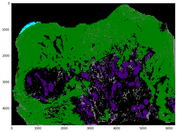
[11]:
# color map
tmp = tissue_pieces[0].labeled.copy()
tmp[0, :256] = np.arange(256)
vals = ['black'] * 256
vals[6] = 'cyan'  # sharpie / ink
vals[7] = 'yellow'  # blood
vals[8] = 'grey'  # whitespace
vals[9] = 'indigo'  # maybe cellular
vals[10] = 'green'  # salient / top cellular
cMap = ListedColormap(vals)

plt.figure(figsize=(10,10))
plt.imshow(tmp, cmap=cMap)
plt.show()
Check the visualization on HistomicsUI
Now you may go to the slide on Digital Slide Archive and check the posted annotations.