Color Deconvolution
Color deconvolution uses color profiles of stains like hematoxylin or diaminobenzidine to digitally separate stains from a color image. This step can help to isolate components like nuclei or positive staining structures which can improve quantitation or other image analysis tasks like segmentation. These examples illustrate how to use HistomicsTK to perform color deconvolution with either known static or adaptive color profiles.
[1]:
from __future__ import print_function

import histomicstk as htk

import numpy as np

import skimage.io
import skimage.measure
import skimage.color

import matplotlib.pyplot as plt
%matplotlib inline

#Some nice default configuration for plots
plt.rcParams['figure.figsize'] = 15, 15
plt.rcParams['image.cmap'] = 'gray'
titlesize = 24
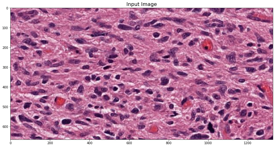
Load input image
HistomicsTK’s color deconvolution routines operate on RGB images, represented as either NxMx3 or 3xN arrays of Numpy’s ndarray type.
[2]:
inputImageFile = ('https://data.kitware.com/api/v1/file/'
                  '57802ac38d777f12682731a2/download')  # H&E.png

imInput = skimage.io.imread(inputImageFile)[:, :, :3]

plt.imshow(imInput)
_ = plt.title('Input Image', fontsize=16)
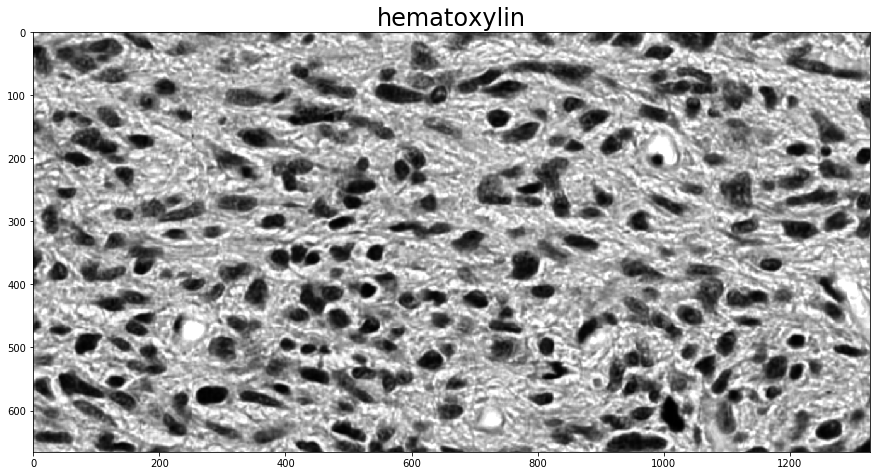
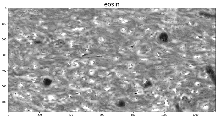
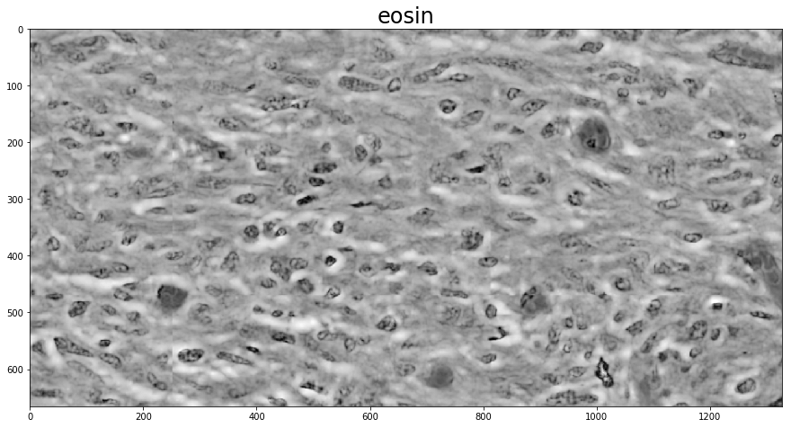
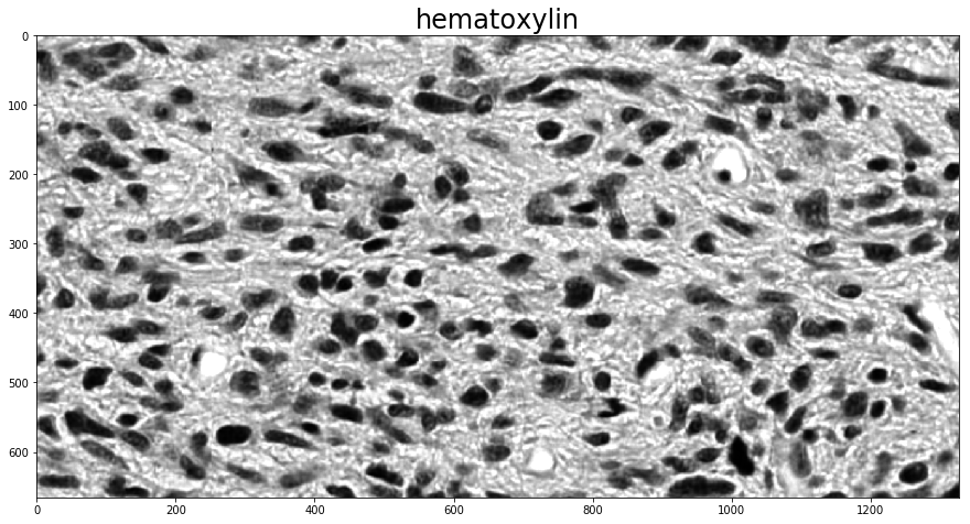
Supervised color deconvolution with a known stain matrix
If you know what the stain matrix to be used for color deconvolution is, computing the deconvolved image is as simple as calling the color_deconvolution function in histomicstk.preprocessing.color_deconvolution. Its input is an RGB image and the stain matrix, and its output is a namedtuple with fields Stains, StainsFloat, and Wc.
Here, we use the built-in stain_color_map dictionary for reference values to fill in the stain matrix. If the image is only two-stain, it makes sense to set the third stain vector perpendicular to the other two, and color_deconvolution does this automatically if the third column is all 0.
[3]:
# create stain to color map
stain_color_map = htk.preprocessing.color_deconvolution.stain_color_map
print('stain_color_map:', stain_color_map, sep='\n')

# specify stains of input image
stains = ['hematoxylin',  # nuclei stain
          'eosin',        # cytoplasm stain
          'null']         # set to null if input contains only two stains

# create stain matrix
W = np.array([stain_color_map[st] for st in stains]).T

# perform standard color deconvolution
imDeconvolved = htk.preprocessing.color_deconvolution.color_deconvolution(imInput, W)

# Display results
for i in 0, 1:
    plt.figure()
    plt.imshow(imDeconvolved.Stains[:, :, i])
    _ = plt.title(stains[i], fontsize=titlesize)
stain_color_map:
{'eosin': [0.07, 0.99, 0.11], 'null': [0.0, 0.0, 0.0], 'hematoxylin': [0.65, 0.7, 0.29], 'dab': [0.27, 0.57, 0.78]}
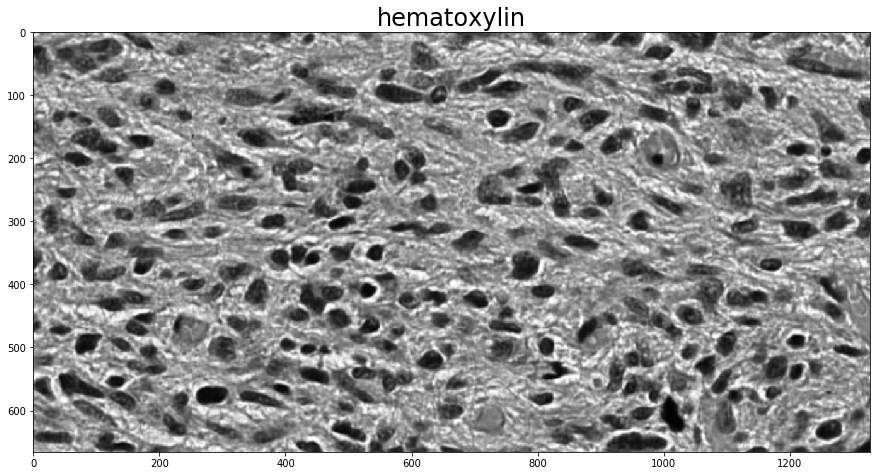
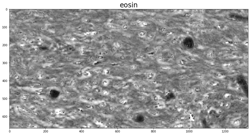
Unsupervised color deconvolution
Sparse non-negative matrix factorization
To determine the stain vectors (somewhat) automatically, HistomicsTK has a couple different methods. The first employs Sparse Non-negative Matrix Factorization (SNMF) to estimate the stain vectors based on an initial guess. Using these methods for color deconvolution then requires two steps, one to calculate the stain vectors with one of the (rgb_)separate_stains_* functions in histomicstk.preprocessing.color_deconvolution and another to apply them to the image with
color_deconvolution.
This example also makes direct use of one of the non-rgb_-prefixed stain-separation functions, which expect an image in the logarithmic SDA space. The conversion to SDA space is done with the rgb_to_sda function in histomicstk.preprocessing.color_conversion. The RGB-to-SDA conversion is parameterized by the background intensity of the image, here called I_0, which we set to 255 (full white; as a scalar it is applied across all channels) as there is no background in the image.
With background available, the function background_intensity in histomicstk.preprocessing.color_normalization can be used to estimate it.
[4]:
# create initial stain matrix
W_init = W[:, :2]

# Compute stain matrix adaptively
sparsity_factor = 0.5

I_0 = 255
im_sda = htk.preprocessing.color_conversion.rgb_to_sda(imInput, I_0)
W_est = htk.preprocessing.color_deconvolution.separate_stains_xu_snmf(
    im_sda, W_init, sparsity_factor,
)

# perform sparse color deconvolution
imDeconvolved = htk.preprocessing.color_deconvolution.color_deconvolution(
    imInput,
    htk.preprocessing.color_deconvolution.complement_stain_matrix(W_est),
    I_0,
)

print('Estimated stain colors (in rows):', W_est.T, sep='\n')

# Display results
for i in 0, 1:
    plt.figure()
    plt.imshow(imDeconvolved.Stains[:, :, i])
    _ = plt.title(stains[i], fontsize=titlesize)
Estimated stain colors (in rows):
[[ 0.48031803  0.78512115  0.39099791]
 [ 0.18892848  0.81830444  0.54284792]]
The PCA-based method of Macenko et al.
Using the rgb_separate_stains_* functions is much the same, except the conversion to SDA space is done as part of the call. The PCA-based routine, unlike the SNMF-based one, does not require an initial guess, and instead automatically determines the vectors of a two-stain image. Because this determination is fully automatic, the order of the stain vector columns in the output is arbitrary. In order to determine which is which, a find_stain_index function is provided in
histomicstk.preprocessing.color_deconvolution that identifies the column in the color deconvolution matrix closest to a given reference vector.
[5]:
w_est = htk.preprocessing.color_deconvolution.rgb_separate_stains_macenko_pca(imInput, I_0)

# Perform color deconvolution
deconv_result = htk.preprocessing.color_deconvolution.color_deconvolution(imInput, w_est, I_0)

print('Estimated stain colors (rows):', w_est.T[:2], sep='\n')

# Display results
for i in 0, 1:
    plt.figure()
    # Unlike SNMF, we're not guaranteed the order of the different stains.
    # find_stain_index guesses which one we want
    channel = htk.preprocessing.color_deconvolution.find_stain_index(
        stain_color_map[stains[i]], w_est)
    plt.imshow(deconv_result.Stains[:, :, channel])
    _ = plt.title(stains[i], fontsize=titlesize)
Estimated stain colors (rows):
[[ 0.16235564  0.81736416  0.55277164]
 [ 0.46329113  0.78963352  0.40229373]]