Converting annotations to object segmentation mask images

Overview:

The DSA database stores annotations in an (x,y) coordinate list format. Some object localization algorithms like Faster-RCNN take coordinate formats whereas others (eg Mask R-CNN) require some form of object segmentation mask image whose pixel values encode not only class but instance information (so that individual objects of the same class can be distinguished).

This notebook demonstrates tools to convert annotations into contours or masks that can be used with algorithms like Mask-RCNN. There are two approaches for generating these data:

• Generate contours or an object segmentation mask image from a region defined by user-specified coordinates.

• Generate contours or object segmentation mask images from annotations contained within region-of-interest (ROI) annotations. This involves mapping annotations to these ROIs and creating one image per ROI.

The examples below extend approaches described in Amgad et al, 2019:

Mohamed Amgad, Habiba Elfandy, Hagar Hussein, …, Jonathan Beezley, Deepak R Chittajallu, David Manthey, David A Gutman, Lee A D Cooper, Structured crowdsourcing enables convolutional segmentation of histology images, Bioinformatics, , btz083, https://doi.org/10.1093/bioinformatics/btz083

A csv file like the one in histomicstk/annotations_and_masks/tests/test_files/sample_GTcodes.csv is needed to define what group each pixel value corresponds to in the mask image, to define the overlay order of various annotation groups, and which groups are considered to be ROIs. Note that the term “group” here comes from the annotation model where each group represents a class like “tumor” or “necrosis” and is associated with a an annotation style.

What is the difference between this and ``annotations_to_masks_handler``?

The difference between this and version 1, found at histomicstk.annotations_and_masks.annotations_to_masks_handler is that this (version 2) gets the contours first, including cropping to wanted ROI boundaries and other processing using shapely, and then parses these into masks. This enables us to differentiate various objects to use the data for object localization/classification/segmentation tasks. If you would like to get semantic segmentation masks instead, i.e. you do not care about individual objects, you can use either version 1 or this handler using the semantic run mode. They re-use much of the same code-base, but some edge cases maybe better handled by version 1. For example, since this version uses shapely first to crop, some objects may be incorrectly parsed by shapely. Version 1, using PIL.ImageDraw may not have these problems.

Bottom line is: if you need semantic segmentation masks, it is probably safer to use version 1 (annotations to masks handler), whereas if you need object segmentation masks, this handler should be used in object run mode.

Where to look?

|_ histomicstk/
  |_annotations_and_masks/
  |  |_annotation_and_mask_utils.py
  |  |_annotations_to_object_mask_handler.py
  |_tests/
      |_ test_annotation_and_mask_utils.py
      |_ test_annotations_to_object_mask_handler.py

import os

import copy
import girder_client
from pandas import DataFrame, read_csv
import tempfile
from imageio import imread
import matplotlib.pyplot as plt
%matplotlib inline

from histomicstk.annotations_and_masks.annotation_and_mask_utils import (
    get_bboxes_from_slide_annotations,
    scale_slide_annotations, get_scale_factor_and_appendStr)
from histomicstk.annotations_and_masks.annotations_to_object_mask_handler import (
    annotations_to_contours_no_mask, contours_to_labeled_object_mask,
    get_all_rois_from_slide_v2)

#Some nice default configuration for plots
plt.rcParams['figure.figsize'] = 7, 7
titlesize = 16

Connect girder client and set parameters

CWD = os.getcwd()

APIURL = 'http://candygram.neurology.emory.edu:8080/api/v1/'
SAMPLE_SLIDE_ID = '5d586d57bd4404c6b1f28640'
GTCODE_PATH = os.path.join(CWD, '../../tests/test_files/sample_GTcodes.csv')

# connect to girder client
gc = girder_client.GirderClient(apiUrl=APIURL)
# gc.authenticate(interactive=True)
gc.authenticate(apiKey='kri19nTIGOkWH01TbzRqfohaaDWb6kPecRqGmemb')

# just a temp directory to save masks for now
BASE_SAVEPATH = tempfile.mkdtemp()
SAVEPATHS = {
    'mask': os.path.join(BASE_SAVEPATH, 'masks'),
    'rgb': os.path.join(BASE_SAVEPATH, 'rgbs'),
    'contours': os.path.join(BASE_SAVEPATH, 'contours'),
    'visualization': os.path.join(BASE_SAVEPATH, 'vis'),
}
for _, savepath in SAVEPATHS.items():
    os.mkdir(savepath)

# What resolution do we want to get the images at?
# Microns-per-pixel / Magnification (either or)
MPP = 2.5  # <- this roughly translates to 4x magnification
MAG = None

Let’s inspect the ground truth codes file

This contains the ground truth codes and information dataframe. This is a dataframe that is indexed by the annotation group name and has the following columns:

• group: group name of annotation (string), eg. “mostly_tumor”

• overlay_order: int, how early to place the annotation in the mask. Larger values means this annotation group is overlayed last and overwrites whatever overlaps it.

• GT_code: int, desired ground truth code (in the labeled mask) Pixels of this value belong to corresponding group (class)

• is_roi: Flag for whether this group marks ‘special’ annotations that encode the ROI boundary

• is_background_class: Flag, whether this group is the default fill value inside the ROI. For example, you may descide that any pixel inside the ROI is considered stroma.

NOTE:

Zero pixels have special meaning and do not encode specific ground truth class. Instead, they simply mean ‘Outside ROI’ and should be ignored during model training or evaluation.

# read GTCodes file
GTCodes_dict = read_csv(GTCODE_PATH)
GTCodes_dict.index = GTCodes_dict.loc[:, 'group']
GTCodes_dict = GTCodes_dict.to_dict(orient='index')

GTCodes_dict.keys()

dict_keys(['roi', 'evaluation_roi', 'mostly_tumor', 'mostly_stroma', 'mostly_lymphocytic_infiltrate', 'necrosis_or_debris', 'glandular_secretions', 'mostly_blood', 'exclude', 'metaplasia_NOS', 'mostly_fat', 'mostly_plasma_cells', 'other_immune_infiltrate', 'mostly_mucoid_material', 'normal_acinus_or_duct', 'lymphatics', 'undetermined', 'nerve', 'skin_adnexia', 'blood_vessel', 'angioinvasion', 'mostly_dcis', 'other'])

GTCodes_dict['mostly_tumor']

{'group': 'mostly_tumor',
 'overlay_order': 1,
 'GT_code': 1,
 'is_roi': 0,
 'is_background_class': 0,
 'color': 'rgb(255,0,0)',
 'comments': 'core class'}

Generate contours for user-defined region

Algorithms like Mask-RCNN consume coordinate data describing the boundaries of objects. The function annotations_to_contours_no_mask generates this countour data for user-specified region. These coordinate data in these contours is relative to the region frame instead of the whole-slide image frame.

print(annotations_to_contours_no_mask.__doc__)

Process annotations to get RGB and contours without intermediate masks.

    Parameters
    ----------
    gc : object
        girder client object to make requests, for example:
        gc = girder_client.GirderClient(apiUrl = APIURL)
        gc.authenticate(interactive=True)

    slide_id : str
        girder id for item (slide)

    MPP : float or None
        Microns-per-pixel -- best use this as it's more well-defined than
        magnification which is more scanner or manufacturer specific.
        MPP of 0.25 often roughly translates to 40x

    MAG : float or None
        If you prefer to use whatever magnification is reported in slide.
        If neither MPP or MAG is provided, everything is retrieved without
        scaling at base (scan) magnification.

    mode : str
        This specifies which part of the slide to get the mask from. Allowed
        modes include the following
        - wsi: get scaled up or down version of mask of whole slide
        - min_bounding_box: get minimum box for all annotations in slide
        - manual_bounds: use given ROI bounds provided by the 'bounds' param
        - polygonal_bounds: use the idx_for_roi param to get coordinates

    bounds : dict or None
        if not None, has keys 'XMIN', 'XMAX', 'YMIN', 'YMAX' for slide
        region coordinates (AT BASE MAGNIFICATION) to get labeled image
        (mask) for. Use this with the 'manual_bounds' run mode.

    idx_for_roi : int
        index of ROI within the element_infos dataframe.
        Use this with the 'polygonal_bounds' run mode.

    slide_annotations : list or None
        Give this parameter to avoid re-getting slide annotations. If you do
        provide the annotations, though, make sure you have used
        scale_slide_annotations() to scale them up or down by sf BEFOREHAND.

    element_infos : pandas DataFrame.
        The columns annidx and elementidx
        encode the dict index of annotation document and element,
        respectively, in the original slide_annotations list of dictionaries.
        This can be obained by get_bboxes_from_slide_annotations() method.
        Make sure you have used scale_slide_annotations().

    linewidth : float
        visualization line width

    get_rgb: bool
        get rgb image?

    get_visualization : bool
        get overlayed annotation bounds over RGB for visualization

    text : bool
        add text labels to visualization?

    Returns
    --------
    dict
        Results dict containing one or more of the following keys
        - bounds: dict of bounds at scan magnification
        - rgb: (mxnx3 np array) corresponding rgb image
        - contours: dict
        - visualization: (mxnx3 np array) visualization overlay

More input parameters

These optional parameters describe the desired magnification or resolution of the output, and whether to generate an RGB image for the region and a visualization image of the annotations.

# common params for annotations_to_contours_no_mask()
annotations_to_contours_kwargs = {
    'MPP': MPP, 'MAG': MAG,
    'linewidth': 0.2,
    'get_rgb': True,
    'get_visualization': True,
    'text': False,
}

1. manual_bounds mode

As shown in the example for generating semantic segmentation masks, this method can be run in four run modes: 1. wsi 2. min_bounding_box 3. manual_bounds 4. polygonal_bounds. Here we test the basic ‘manual_bounds’ mode where the boundaries of the region you want are provided at base/scan magnification.

bounds = {
    'XMIN': 58000, 'XMAX': 63000,
    'YMIN': 35000, 'YMAX': 39000,
}

# get specified region, let the method get and scale annotations
roi_out = annotations_to_contours_no_mask(
    gc=gc, slide_id=SAMPLE_SLIDE_ID,
    mode='manual_bounds', bounds=bounds,
    **annotations_to_contours_kwargs)

/home/mtageld/Desktop/HistomicsTK/histomicstk/annotations_and_masks/annotation_and_mask_utils.py:668: RuntimeWarning: invalid value encountered in greater
  iou = iou[:, iou[1, :] > iou_thresh].astype(int)

The result is an rgb image, contours and a visualization. Let’s take a look at these below.

roi_out.keys()

dict_keys(['rgb', 'contours', 'bounds', 'visualization'])

roi_out['bounds']

{'XMIN': 57994, 'XMAX': 62994, 'YMIN': 34999, 'YMAX': 38992}

for imstr in ['rgb', 'visualization']:
    plt.imshow(roi_out[imstr])
    plt.title(imstr)
    plt.show()

DataFrame(roi_out['contours']).head()

	annidx	annotation_girder_id	elementidx	element_girder_id	type	group	label	color	xmin	xmax	ymin	ymax	bbox_area	coords_x	coords_y
0	0	5d586d58bd4404c6b1f28642	0	5a943eb992ca9a0016fae97f	rectangle	roi	roi	rgb(163, 19, 186)	121	501	0	310	117800	491,143,121,292,501,501,491	0,0,13,310,189,15,0
1	1	5d586d58bd4404c6b1f28644	0	5a943eb992ca9a0016fae981	polyline	blood_vessel	blood_vessel	rgb(128,0,128)	341	360	241	259	342	353,352,351,350,350,349,348,347,346,345,344,34...	241,241,241,241,242,242,242,242,242,242,242,24...
2	1	5d586d58bd4404c6b1f28644	1	5a943eb992ca9a0016fae982	polyline	blood_vessel	blood_vessel	rgb(128,0,128)	244	258	161	181	280	244,244,244,244,244,244,245,245,245,245,245,24...	161,162,163,165,166,167,167,168,169,170,171,17...
3	2	5d586d58bd4404c6b1f2864c	0	5a943eba92ca9a0016fae990	polyline	mostly_lymphocytic_infiltrate	mostly_lymphocytic_infiltrate	rgb(0,0,255)	388	501	71	236	18645	501,501,500,500,499,498,498,497,496,495,495,49...	171,75,75,74,74,74,73,73,72,72,71,71,71,71,72,...
4	2	5d586d58bd4404c6b1f2864c	1	5a943eba92ca9a0016fae994	polyline	mostly_lymphocytic_infiltrate	mostly_lymphocytic_infiltrate	rgb(0,0,255)	359	434	0	21	1575	434,359,359,359,360,360,360,361,361,362,362,36...	0,0,1,2,2,3,4,5,6,6,7,7,7,7,7,8,8,8,9,9,11,12,...

Note that if the above function call is made repeatedly for the same slide (e.g. to iterate over multiple regions), multiple get requests would be created to retrieve annotations from the server. To improve efficiency when handling multiple regions in the same slide, we could manually get annotations and scale them down/up to desired resolution, and pass them to annotations_to_contours_no_mask().

# get annotations for slide
slide_annotations = gc.get('/annotation/item/' + SAMPLE_SLIDE_ID)

# scale up/down annotations by a factor
sf, _ = get_scale_factor_and_appendStr(
    gc=gc, slide_id=SAMPLE_SLIDE_ID, MPP=MPP, MAG=MAG)
slide_annotations = scale_slide_annotations(slide_annotations, sf=sf)

# get bounding box information for all annotations
element_infos = get_bboxes_from_slide_annotations(slide_annotations)

# get specified region -- manually providing scaled annotations
roi_out = annotations_to_contours_no_mask(
    gc=gc, slide_id=SAMPLE_SLIDE_ID,
    mode='manual_bounds', bounds=bounds,
    slide_annotations=slide_annotations, element_infos=element_infos,
    **annotations_to_contours_kwargs)

/home/mtageld/Desktop/HistomicsTK/histomicstk/annotations_and_masks/annotation_and_mask_utils.py:668: RuntimeWarning: invalid value encountered in greater
  iou = iou[:, iou[1, :] > iou_thresh].astype(int)

roi_out['bounds']

{'XMIN': 57994, 'XMAX': 62994, 'YMIN': 34999, 'YMAX': 38992}

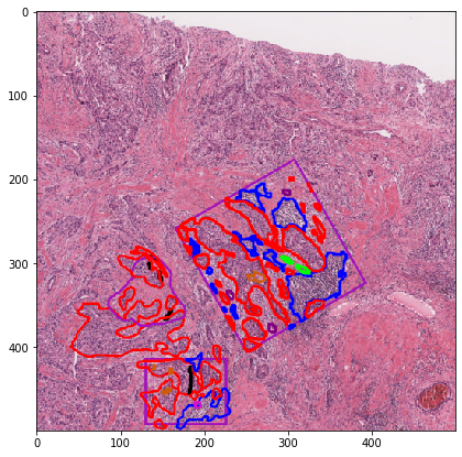
2. min_bounding_box mode

In min_bounding_box mode everything in the slide is handled using the smallest rectangular bounding box.

# get ROI bounding everything
minbbox_out = annotations_to_contours_no_mask(
    gc=gc, slide_id=SAMPLE_SLIDE_ID,
    mode='min_bounding_box', **annotations_to_contours_kwargs)

minbbox_out['bounds']

{'XMIN': 56726, 'YMIN': 33483, 'XMAX': 63732, 'YMAX': 39890}

plt.imshow(minbbox_out['visualization'])

<matplotlib.image.AxesImage at 0x7f1825c3f8d0>

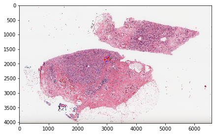
3. wsi mode

wsi mode creates a scaled version of the entire whole-slide image and all annotations contained within.

NOTE:

This does not rely on tiles and processes the image at whatever magnification you want. You can supress the RGB or visualization outputs and to just fetch the contours or object segmentation mask (see below), providing a bigger magnification range before encountering memory problems.

# get entire wsi region
get_kwargs = copy.deepcopy(annotations_to_contours_kwargs)
get_kwargs['MPP'] = 5.0  # otherwise it's too large!
wsi_out = annotations_to_contours_no_mask(
    gc=gc, slide_id=SAMPLE_SLIDE_ID,
    mode='wsi', **get_kwargs)

wsi_out['bounds']

{'XMIN': 0, 'XMAX': 131516, 'YMIN': 0, 'YMAX': 80439}

plt.imshow(wsi_out['visualization'])
plt.show()

plt.imshow(wsi_out['visualization'][1500:2000, 2800:3300])
plt.show()

Parse manually-drawn ROIs into separate labeled object masks

This function utilizes the polygonal_bounds mode of the get_image_and_mask_from_slide() method to generate a set of outputs for each ROI annotation.

In the example above we focused on generating contour data to represent objects. Below we focus on generating object segmentation mask images.

print(get_all_rois_from_slide_v2.__doc__)

Get all ROIs for a slide without an intermediate mask form.

    This mainly relies on contours_to_labeled_object_mask(), which should
    be referred to for extra documentation.

    This can be run in either the "object" mode, whereby the saved masks
    are a three-channel png where first channel encodes class label (i.e.
    same as semantic segmentation) and the product of the values in the
    second and third channel encodes the object ID. Otherwise, the user
    may decide to run in the "semantic" mode and the resultant mask would
    consist of only one channel (semantic segmentation with no object
    differentiation).

    The difference between this and version 1, found at
    histomicstk.annotations_and_masks.annotations_to_masks_handler.
    get_all_rois_from_slide()
    is that this (version 2) gets the contours first, including cropping
    to wanted ROI boundaries and other processing using shapely, and THEN
    parses these into masks. This enables us to differentiate various objects
    to use the data for object localization or classification or segmentation
    tasks. If you would like to get semantic segmentation masks, i.e. you do
    not really care about individual objects, you can use either version 1
    or this method. They re-use much of the same code-base, but some edge
    cases maybe better handled by version 1. For example, since
    this version uses shapely first to crop, some objects may be incorrectly
    parsed by shapely. Version 1, using PIL.ImageDraw may not have these
    problems.

    Bottom line is: if you need semantic segmentation masks, it is probably
    safer to use version 1, whereas if you need object segmentation masks,
    this method should be used.

    Parameters
    ----------
    gc : object
        girder client object to make requests, for example:
        gc = girder_client.GirderClient(apiUrl = APIURL)
        gc.authenticate(interactive=True)

    slide_id : str
        girder id for item (slide)

    GTCodes_dict : dict
        the ground truth codes and information dict.
        This is a dict that is indexed by the annotation group name and
        each entry is in turn a dict with the following keys:
        - group: group name of annotation (string), eg. mostly_tumor
        - overlay_order: int, how early to place the annotation in the
        mask. Larger values means this annotation group is overlayed
        last and overwrites whatever overlaps it.
        - GT_code: int, desired ground truth code (in the mask)
        Pixels of this value belong to corresponding group (class)
        - is_roi: Flag for whether this group encodes an ROI
        - is_background_class: Flag, whether this group is the default
        fill value inside the ROI. For example, you may descide that
        any pixel inside the ROI is considered stroma.

    save_directories : dict
        paths to directories to save data. Each entry is a string, and the
        following keys are allowed
        - ROI: path to save masks (labeled images)
        - rgb: path to save rgb images
        - contours: path to save annotation contours
        - visualization: path to save rgb visualzation overlays

    mode : str
        run mode for getting masks. Must me in
        - object: get 3-channel mask where first channel encodes label
        (tumor, stroma, etc) while product of second and third
        channel encodes the object ID (i.e. individual contours)
        This is useful for object localization and segmentation tasks.
        - semantic: get a 1-channel mask corresponding to the first channel
        of the object mode.

    get_mask : bool
        While the main purpose of this method IS to get object segmentation
        masks, it is conceivable that some users might just want to get
        the RGB and contours. Default is True.

    annotations_to_contours_kwargs : dict
        kwargs to pass to annotations_to_contours_no_mask()
        default values are assigned if specific parameters are not given.

    slide_name : str or None
        If not given, its inferred using a server request using girder client.

    verbose : bool
        Print progress to screen?

    monitorprefix : str
        text to prepend to printed statements

    callback : function
        a callback function to run on the roi dictionary output. This is
        internal, but if you really want to use this, make sure the callback
        can accept the following keys and that you do NOT assign them yourself
        gc, slide_id, slide_name, MPP, MAG, verbose, monitorprefix
        Also, this callback MUST *ONLY* return thr roi dictionary, whether
        or not it is modified inside it. If it is modified inside the callback
        then the modified version is the one that will be saved to disk.

    callback_kwargs : dict
        kwargs to pass to callback, not including the mandatory kwargs
        that will be passed internally (mentioned earlier here).

    Returns
    --------
    list of dicts
        each entry contains the following keys
        mask - path to saved mask
        rgb - path to saved rgb image
        contours - path to saved annotation contours
        visualization - path to saved rgb visualzation overlay

The above method mainly relies on contours_to_labeled_object_mask(), described below.

print(contours_to_labeled_object_mask.__doc__)

Process contours to get and object segmentation labeled mask.

    Parameters
    ----------
    contours : DataFrame
        contours corresponding to annotation elemeents from the slide.
        All coordinates are relative to the mask that you want to output.
        The following columns are expected.
        - group: str, annotation group (ground truth label).
        - ymin: int, minimun y coordinate
        - ymax: int, maximum y coordinate
        - xmin: int, minimum x coordinate
        - xmax: int, maximum x coordinate
        - coords_x: str, vertix x coordinates comma-separated values
        - coords_y: str, vertix y coordinated comma-separated values

    gtcodes : DataFrame
        the ground truth codes and information dataframe.
        This is a dataframe that is indexed by the annotation group name
        and has the following columns.
        - group: str, group name of annotation, eg. mostly_tumor.
        - GT_code: int, desired ground truth code (in the mask).
        Pixels of this value belong to corresponding group (class).
        - color: str, rgb format. eg. rgb(255,0,0).

    mode : str
        run mode for getting masks. Must be in
        - object: get 3-channel mask where first channel encodes label
        (tumor, stroma, etc) while product of second and third
        channel encodes the object ID (i.e. individual contours)
        This is useful for object localization and segmentation tasks.
        - semantic: get a 1-channel mask corresponding to the first channel
        of the object mode.

    verbose : bool
        print to screen?

    monitorprefix : str
        prefix to add to printed statemens

    Returns
    -------
    np.array
        If mode is "object", this returns an (m, n, 3) np array
        that can be saved as a png
        First channel: encodes label (can be used for semantic segmentation)
        Second & third channels: multiplication of second and third channel
        gives the object id (255 choose 2 = 32,385 max unique objects).
        This allows us to save into a convenient 3-channel png object labels
        and segmentation masks, which is more compact than traditional
        mask-rcnn save formats like having one channel per object and a
        separate csv file for object labels. This is also more convenient
        than simply saving things into pickled np array objects, and allows
        compatibility with data loaders that expect an image or mask.
        If mode is "semantic" only the labels (corresponding to first
        channel of the object mode) is output.

get_all_rois_kwargs = {
    'gc': gc,
    'slide_id': SAMPLE_SLIDE_ID,
    'GTCodes_dict': GTCodes_dict,
    'save_directories': SAVEPATHS,
    'annotations_to_contours_kwargs': annotations_to_contours_kwargs,
    'slide_name': 'TCGA-A2-A0YE',
    'mode': 'object',
    'verbose': True,
    'monitorprefix': 'test',
}
savenames = get_all_rois_from_slide_v2(**get_all_rois_kwargs)

test: roi 1 of 3: Overlay level -1: Element 1 of 50: roi
test: roi 1 of 3: Overlay level 1: Element 2 of 50: mostly_tumor
test: roi 1 of 3: Overlay level 1: Element 3 of 50: mostly_lymphocytic_infiltrate
test: roi 1 of 3: Overlay level 1: Element 4 of 50: mostly_tumor
test: roi 1 of 3: Overlay level 1: Element 5 of 50: mostly_tumor
test: roi 1 of 3: Overlay level 1: Element 6 of 50: mostly_lymphocytic_infiltrate
test: roi 1 of 3: Overlay level 1: Element 7 of 50: mostly_lymphocytic_infiltrate
test: roi 1 of 3: Overlay level 1: Element 8 of 50: mostly_lymphocytic_infiltrate
test: roi 1 of 3: Overlay level 1: Element 9 of 50: mostly_tumor
test: roi 1 of 3: Overlay level 1: Element 10 of 50: mostly_lymphocytic_infiltrate
test: roi 1 of 3: Overlay level 1: Element 11 of 50: mostly_tumor
test: roi 1 of 3: Overlay level 1: Element 12 of 50: mostly_tumor
test: roi 1 of 3: Overlay level 1: Element 13 of 50: mostly_tumor
test: roi 1 of 3: Overlay level 1: Element 14 of 50: mostly_tumor
test: roi 1 of 3: Overlay level 1: Element 15 of 50: mostly_lymphocytic_infiltrate
test: roi 1 of 3: Overlay level 1: Element 16 of 50: mostly_tumor
test: roi 1 of 3: Overlay level 1: Element 17 of 50: mostly_lymphocytic_infiltrate
test: roi 1 of 3: Overlay level 1: Element 18 of 50: mostly_tumor
test: roi 1 of 3: Overlay level 1: Element 19 of 50: mostly_tumor
test: roi 1 of 3: Overlay level 1: Element 20 of 50: mostly_tumor
test: roi 1 of 3: Overlay level 1: Element 21 of 50: mostly_tumor
test: roi 1 of 3: Overlay level 1: Element 22 of 50: mostly_tumor
test: roi 1 of 3: Overlay level 1: Element 23 of 50: normal_acinus_or_duct
test: roi 1 of 3: Overlay level 1: Element 24 of 50: mostly_tumor
test: roi 1 of 3: Overlay level 1: Element 25 of 50: normal_acinus_or_duct
test: roi 1 of 3: Overlay level 1: Element 26 of 50: mostly_lymphocytic_infiltrate
test: roi 1 of 3: Overlay level 1: Element 27 of 50: mostly_tumor
test: roi 1 of 3: Overlay level 1: Element 28 of 50: blood_vessel
test: roi 1 of 3: Overlay level 1: Element 29 of 50: mostly_lymphocytic_infiltrate
test: roi 1 of 3: Overlay level 1: Element 30 of 50: blood_vessel
test: roi 1 of 3: Overlay level 1: Element 31 of 50: blood_vessel
test: roi 1 of 3: Overlay level 1: Element 32 of 50: mostly_tumor
test: roi 1 of 3: Overlay level 1: Element 33 of 50: mostly_tumor
test: roi 1 of 3: Overlay level 1: Element 34 of 50: mostly_tumor
test: roi 1 of 3: Overlay level 1: Element 35 of 50: mostly_lymphocytic_infiltrate
test: roi 1 of 3: Overlay level 1: Element 36 of 50: mostly_lymphocytic_infiltrate
test: roi 1 of 3: Overlay level 1: Element 37 of 50: mostly_tumor
test: roi 1 of 3: Overlay level 1: Element 38 of 50: mostly_tumor
test: roi 1 of 3: Overlay level 1: Element 39 of 50: mostly_tumor
test: roi 1 of 3: Overlay level 1: Element 40 of 50: mostly_tumor
test: roi 1 of 3: Overlay level 1: Element 41 of 50: mostly_lymphocytic_infiltrate
test: roi 1 of 3: Overlay level 1: Element 42 of 50: mostly_tumor
test: roi 1 of 3: Overlay level 1: Element 43 of 50: mostly_lymphocytic_infiltrate
test: roi 1 of 3: Overlay level 1: Element 44 of 50: mostly_tumor
test: roi 1 of 3: Overlay level 1: Element 45 of 50: mostly_tumor
test: roi 1 of 3: Overlay level 1: Element 46 of 50: mostly_lymphocytic_infiltrate
test: roi 1 of 3: Overlay level 1: Element 47 of 50: mostly_lymphocytic_infiltrate
test: roi 1 of 3: Overlay level 1: Element 48 of 50: mostly_tumor
test: roi 1 of 3: Overlay level 2: Element 49 of 50: mostly_stroma
test: roi 1 of 3: Overlay level 3: Element 50 of 50: exclude
test: roi 1 of 3: Saving /tmp/tmpvdwsnssq/masks/TCGA-A2-A0YE_left-59191_top-33483_bottom-38083_right-63732.png
test: roi 1 of 3: Saving /tmp/tmpvdwsnssq/rgbs/TCGA-A2-A0YE_left-59191_top-33483_bottom-38083_right-63732.png
test: roi 1 of 3: Saving /tmp/tmpvdwsnssq/vis/TCGA-A2-A0YE_left-59191_top-33483_bottom-38083_right-63732.png
test: roi 1 of 3: Saving /tmp/tmpvdwsnssq/contours/TCGA-A2-A0YE_left-59191_top-33483_bottom-38083_right-63732.csv

test: roi 2 of 3: Overlay level -2: Element 1 of 16: roi
test: roi 2 of 3: Overlay level 1: Element 2 of 16: mostly_tumor
test: roi 2 of 3: Overlay level 1: Element 3 of 16: mostly_lymphocytic_infiltrate
test: roi 2 of 3: Overlay level 1: Element 4 of 16: mostly_tumor
test: roi 2 of 3: Overlay level 1: Element 5 of 16: mostly_tumor
test: roi 2 of 3: Overlay level 1: Element 6 of 16: mostly_lymphocytic_infiltrate
test: roi 2 of 3: Overlay level 1: Element 7 of 16: mostly_tumor
test: roi 2 of 3: Overlay level 1: Element 8 of 16: mostly_tumor
test: roi 2 of 3: Overlay level 1: Element 9 of 16: blood_vessel
test: roi 2 of 3: Overlay level 1: Element 10 of 16: mostly_tumor
test: roi 2 of 3: Overlay level 1: Element 11 of 16: mostly_tumor
test: roi 2 of 3: Overlay level 1: Element 12 of 16: mostly_tumor
test: roi 2 of 3: Overlay level 2: Element 13 of 16: mostly_stroma
test: roi 2 of 3: Overlay level 2: Element 14 of 16: mostly_stroma
test: roi 2 of 3: Overlay level 2: Element 15 of 16: mostly_stroma
test: roi 2 of 3: Overlay level 3: Element 16 of 16: exclude
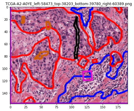
test: roi 2 of 3: Saving /tmp/tmpvdwsnssq/masks/TCGA-A2-A0YE_left-58473_top-38203_bottom-39780_right-60389.png
test: roi 2 of 3: Saving /tmp/tmpvdwsnssq/rgbs/TCGA-A2-A0YE_left-58473_top-38203_bottom-39780_right-60389.png
test: roi 2 of 3: Saving /tmp/tmpvdwsnssq/vis/TCGA-A2-A0YE_left-58473_top-38203_bottom-39780_right-60389.png
test: roi 2 of 3: Saving /tmp/tmpvdwsnssq/contours/TCGA-A2-A0YE_left-58473_top-38203_bottom-39780_right-60389.csv

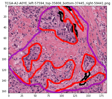
test: roi 3 of 3: Overlay level -3: Element 1 of 11: roi
test: roi 3 of 3: Overlay level 1: Element 2 of 11: mostly_tumor
test: roi 3 of 3: Overlay level 1: Element 3 of 11: mostly_tumor
test: roi 3 of 3: Overlay level 1: Element 4 of 11: mostly_tumor
test: roi 3 of 3: Overlay level 1: Element 5 of 11: mostly_tumor
test: roi 3 of 3: Overlay level 1: Element 6 of 11: mostly_tumor
test: roi 3 of 3: Overlay level 1: Element 7 of 11: mostly_tumor
test: roi 3 of 3: Overlay level 3: Element 8 of 11: exclude
test: roi 3 of 3: Overlay level 3: Element 9 of 11: exclude
test: roi 3 of 3: Overlay level 3: Element 10 of 11: exclude
test: roi 3 of 3: Overlay level 3: Element 11 of 11: exclude
test: roi 3 of 3: Saving /tmp/tmpvdwsnssq/masks/TCGA-A2-A0YE_left-57594_top-35808_bottom-37445_right-59441.png
test: roi 3 of 3: Saving /tmp/tmpvdwsnssq/rgbs/TCGA-A2-A0YE_left-57594_top-35808_bottom-37445_right-59441.png
test: roi 3 of 3: Saving /tmp/tmpvdwsnssq/vis/TCGA-A2-A0YE_left-57594_top-35808_bottom-37445_right-59441.png
test: roi 3 of 3: Saving /tmp/tmpvdwsnssq/contours/TCGA-A2-A0YE_left-57594_top-35808_bottom-37445_right-59441.csv

savenames[0]

{'mask': '/tmp/tmpvdwsnssq/masks/TCGA-A2-A0YE_left-59191_top-33483_bottom-38083_right-63732.png',
 'rgb': '/tmp/tmpvdwsnssq/rgbs/TCGA-A2-A0YE_left-59191_top-33483_bottom-38083_right-63732.png',
 'visualization': '/tmp/tmpvdwsnssq/vis/TCGA-A2-A0YE_left-59191_top-33483_bottom-38083_right-63732.png',
 'contours': '/tmp/tmpvdwsnssq/contours/TCGA-A2-A0YE_left-59191_top-33483_bottom-38083_right-63732.csv'}

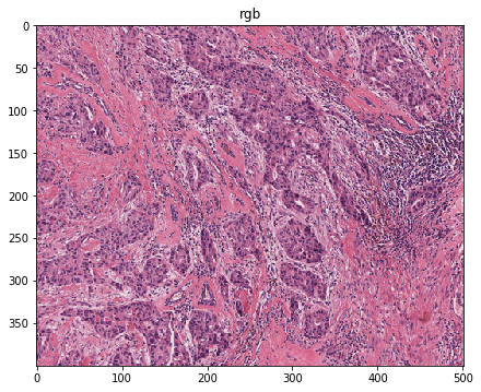
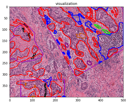
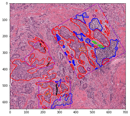
Let’s visualize the contours

# visualization of contours over RGBs
for savename in savenames:
    vis = imread(savename['visualization'])
    plt.imshow(vis)
    plt.title(os.path.basename(savename['visualization']))
    plt.show()

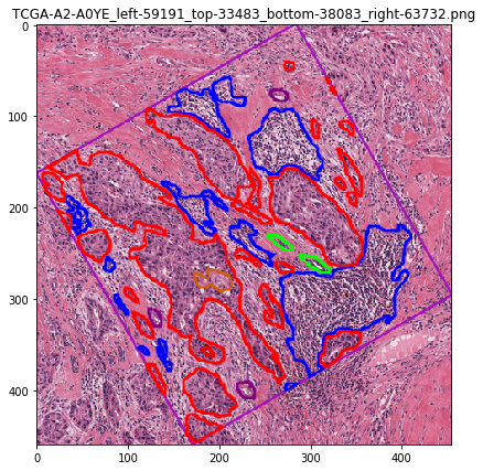
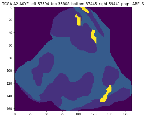
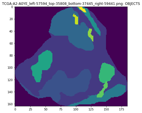
Let’s visualize the object mask

An object segmentation mask image uses the multiple channels to encode both class and instance information. In this mask format we multiply the second and third channel values to calculate a unique id for each object.

mask = imread(savename['mask'])
maskname = os.path.basename(savename['mask'])

plt.imshow(mask[..., 0])
plt.title(maskname + ': LABELS')
plt.show()

plt.imshow(mask[..., 1] * mask[..., 2])
plt.title(maskname + ': OBJECTS')
plt.show()